目录
简介
导入
层刻度层
随机深度层
类注意力
会说话的头注意力
前馈网络
其他模块
拼凑碎片:CaiT 模型
定义模型配置
模型实例化
加载预训练模型
推理工具
加载图像
获取预测
关注层可视化
结论
政安晨的个人主页:政安晨
欢迎 👍点赞✍评论⭐收藏
收录专栏: TensorFlow与Keras机器学习实战
希望政安晨的博客能够对您有所裨益,如有不足之处,欢迎在评论区提出指正!
本文目标:实现配备关注类和 LayerScale 的图像转换器。
简介
在本文中,我们将实现 Touvron 等人在《深入研究图像变换器》(Going deeper with Image Transformers)一书中提出的 CaiT(Class-Attention in Image Transformers)。
深度缩放,即增加模型深度以获得更好的性能和泛化,在卷积神经网络(例如 Tan 等人,Dollár 等人)中已经取得了相当大的成功。但是,将相同的模型缩放原则应用于视觉转换器(Dosovitskiy 等人)并不能获得同样好的效果--它们的性能会随着深度缩放而迅速饱和。
请注意,这里的一个假设是,在进行模型缩放时,基础预训练数据集始终保持固定。
在 CaiT 论文中,作者对这一现象进行了研究,并提出了修改 ViT(视觉转换器)架构的建议,以缓解这一问题。
这样的教程结构是这样的:
—— 实现 CaiT 的各个模块
—— 整理所有模块以创建 CaiT 模型
—— 加载预训练的 CaiT 模型
—— 获取预测结果
—— CaiT 不同注意层的可视化
假定读者已经熟悉视觉转换器。
下面是视觉转换器在 Keras 中的实现:使用视觉转换器进行图像分类。
导入
import os

os.environ["KERAS_BACKEND"] = "tensorflow"

import io
import typing
from urllib.request import urlopen

import matplotlib.pyplot as plt
import numpy as np
import PIL
import keras
from keras import layers
from keras import ops
层刻度层
我们首先要实现一个 LayerScale 层,它是 CaiT 论文中提出的两个修改方案之一。
当增加 ViT 模型的深度时,它们会遇到优化不稳定的问题,最终无法收敛。每个变换器块内的残余连接带来了信息瓶颈。当深度增加时,这一瓶颈会迅速爆发,并偏离基础模型的优化路径。
以下公式表示在变压器模块内添加剩余连接的位置:
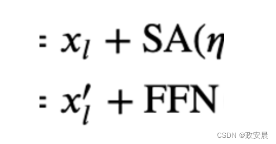
其中,SA 表示自我注意,FFN 表示前馈网络,eta 表示层规范算子(Ba 等人)。
LayerScale 的形式是这样实现的:
其中,lambdas 是可学习参数,初始化值很小({0.1, 1e-5, 1e-6})。 diag 表示对角矩阵。
直观地说,LayerScale 有助于控制残余分支的贡献。LayerScale 的可学习参数被初始化为一个较小的值,让分支像身份函数一样行动,然后让它们在训练过程中找出交互程度。对角矩阵还有助于控制残差输入各个维度的贡献,因为它是按通道应用的。
LayerScale 的实际实现比听起来要简单得多。
class LayerScale(layers.Layer):
    """LayerScale as introduced in CaiT: https://arxiv.org/abs/2103.17239.

    Args:
        init_values (float): value to initialize the diagonal matrix of LayerScale.
        projection_dim (int): projection dimension used in LayerScale.
    """

    def __init__(self, init_values: float, projection_dim: int, **kwargs):
        super().__init__(**kwargs)
        self.gamma = self.add_weight(
            shape=(projection_dim,),
            initializer=keras.initializers.Constant(init_values),
        )

    def call(self, x, training=False):
        return x * self.gamma
随机深度层
随机深度层自问世以来(Huang 等人),已成为几乎所有现代神经网络架构中最受欢迎的组件。CaiT 也不例外。
讨论随机深度层超出了本笔记本的范围。如果您需要复习,可以参考本资料。
class StochasticDepth(layers.Layer):
    """Stochastic Depth layer (https://arxiv.org/abs/1603.09382).

    Reference:
        https://github.com/rwightman/pytorch-image-models
    """

    def __init__(self, drop_prob: float, **kwargs):
        super().__init__(**kwargs)
        self.drop_prob = drop_prob
        self.seed_generator = keras.random.SeedGenerator(1337)

    def call(self, x, training=False):
        if training:
            keep_prob = 1 - self.drop_prob
            shape = (ops.shape(x)[0],) + (1,) * (len(x.shape) - 1)
            random_tensor = keep_prob + ops.random.uniform(
                shape, minval=0, maxval=1, seed=self.seed_generator
            )
            random_tensor = ops.floor(random_tensor)
            return (x / keep_prob) * random_tensor
        return x
类注意力
vanilla ViT 使用自我注意(SA)层来模拟图像补丁和可学习 CLS 标记之间的相互作用。CaiT 的作者建议将负责关注图像斑块和 CLS 标记的注意层分离开来。
在使用 ViT 执行任何辨别任务(例如分类)时,我们通常会使用属于 CLS 标记的表征,然后将其传递给特定任务的头部。这有别于卷积神经网络中通常采用的全局平均池化方法。
CLS 标记与其他图像斑块之间的相互作用是通过自我注意层统一处理的。正如 CaiT 的作者所指出的,这种设置产生了纠缠不清的效果。一方面,自我注意层负责图像补丁的建模。另一方面,它们还负责通过 CLS 标记总结建模信息,以便对学习目标有用。
为了帮助厘清这两件事,作者建议:
在网络的后期阶段引入 CLS 标记。
通过一组独立的注意层来模拟 CLS 标记与图像补丁相关表征之间的互动。作者称之为 "类注意力"(CA)。
这是通过将 CLS 标记嵌入作为 CA 层中的查询来实现的。CLS 标记嵌入和图像补丁嵌入既是键,也是值。
请注意,这里的 "嵌入 "和 "表征 "可以互换使用。
class ClassAttention(layers.Layer):
    """Class attention as proposed in CaiT: https://arxiv.org/abs/2103.17239.

    Args:
        projection_dim (int): projection dimension for the query, key, and value
            of attention.
        num_heads (int): number of attention heads.
        dropout_rate (float): dropout rate to be used for dropout in the attention
            scores as well as the final projected outputs.
    """

    def __init__(
        self, projection_dim: int, num_heads: int, dropout_rate: float, **kwargs
    ):
        super().__init__(**kwargs)
        self.num_heads = num_heads

        head_dim = projection_dim // num_heads
        self.scale = head_dim**-0.5

        self.q = layers.Dense(projection_dim)
        self.k = layers.Dense(projection_dim)
        self.v = layers.Dense(projection_dim)
        self.attn_drop = layers.Dropout(dropout_rate)
        self.proj = layers.Dense(projection_dim)
        self.proj_drop = layers.Dropout(dropout_rate)

    def call(self, x, training=False):
        batch_size, num_patches, num_channels = (
            ops.shape(x)[0],
            ops.shape(x)[1],
            ops.shape(x)[2],
        )

        # Query projection. `cls_token` embeddings are queries.
        q = ops.expand_dims(self.q(x[:, 0]), axis=1)
        q = ops.reshape(
            q, (batch_size, 1, self.num_heads, num_channels // self.num_heads)
        )  # Shape: (batch_size, 1, num_heads, dimension_per_head)
        q = ops.transpose(q, axes=[0, 2, 1, 3])
        scale = ops.cast(self.scale, dtype=q.dtype)
        q = q * scale

        # Key projection. Patch embeddings as well the cls embedding are used as keys.
        k = self.k(x)
        k = ops.reshape(
            k, (batch_size, num_patches, self.num_heads, num_channels // self.num_heads)
        )  # Shape: (batch_size, num_tokens, num_heads, dimension_per_head)
        k = ops.transpose(k, axes=[0, 2, 3, 1])

        # Value projection. Patch embeddings as well the cls embedding are used as values.
        v = self.v(x)
        v = ops.reshape(
            v, (batch_size, num_patches, self.num_heads, num_channels // self.num_heads)
        )
        v = ops.transpose(v, axes=[0, 2, 1, 3])

        # Calculate attention scores between cls_token embedding and patch embeddings.
        attn = ops.matmul(q, k)
        attn = ops.nn.softmax(attn, axis=-1)
        attn = self.attn_drop(attn, training=training)

        x_cls = ops.matmul(attn, v)
        x_cls = ops.transpose(x_cls, axes=[0, 2, 1, 3])
        x_cls = ops.reshape(x_cls, (batch_size, 1, num_channels))
        x_cls = self.proj(x_cls)
        x_cls = self.proj_drop(x_cls, training=training)

        return x_cls, attn
会说话的头注意力
CaiT 的作者使用 Talking Head Attention(Shazeer 等人)取代了最初 Transformer 论文(Vaswani 等人)中使用的 vanilla scaled dot-product multi-head Attention。他们在软最大运算前后引入了两个线性投影,以获得更好的效果。
有关 Talking Head 注意力和 vanilla 注意力机制的更严谨的论述,请参阅他们各自的论文(如上链接)。
class TalkingHeadAttention(layers.Layer):
    """Talking-head attention as proposed in CaiT: https://arxiv.org/abs/2003.02436.

    Args:
        projection_dim (int): projection dimension for the query, key, and value
            of attention.
        num_heads (int): number of attention heads.
        dropout_rate (float): dropout rate to be used for dropout in the attention
            scores as well as the final projected outputs.
    """

    def __init__(
        self, projection_dim: int, num_heads: int, dropout_rate: float, **kwargs
    ):
        super().__init__(**kwargs)

        self.num_heads = num_heads

        head_dim = projection_dim // self.num_heads

        self.scale = head_dim**-0.5

        self.qkv = layers.Dense(projection_dim * 3)
        self.attn_drop = layers.Dropout(dropout_rate)

        self.proj = layers.Dense(projection_dim)

        self.proj_l = layers.Dense(self.num_heads)
        self.proj_w = layers.Dense(self.num_heads)

        self.proj_drop = layers.Dropout(dropout_rate)

    def call(self, x, training=False):
        B, N, C = ops.shape(x)[0], ops.shape(x)[1], ops.shape(x)[2]

        # Project the inputs all at once.
        qkv = self.qkv(x)

        # Reshape the projected output so that they're segregated in terms of
        # query, key, and value projections.
        qkv = ops.reshape(qkv, (B, N, 3, self.num_heads, C // self.num_heads))

        # Transpose so that the `num_heads` becomes the leading dimensions.
        # Helps to better segregate the representation sub-spaces.
        qkv = ops.transpose(qkv, axes=[2, 0, 3, 1, 4])
        scale = ops.cast(self.scale, dtype=qkv.dtype)
        q, k, v = qkv[0] * scale, qkv[1], qkv[2]

        # Obtain the raw attention scores.
        attn = ops.matmul(q, ops.transpose(k, axes=[0, 1, 3, 2]))

        # Linear projection of the similarities between the query and key projections.
        attn = self.proj_l(ops.transpose(attn, axes=[0, 2, 3, 1]))

        # Normalize the attention scores.
        attn = ops.transpose(attn, axes=[0, 3, 1, 2])
        attn = ops.nn.softmax(attn, axis=-1)

        # Linear projection on the softmaxed scores.
        attn = self.proj_w(ops.transpose(attn, axes=[0, 2, 3, 1]))
        attn = ops.transpose(attn, axes=[0, 3, 1, 2])
        attn = self.attn_drop(attn, training=training)

        # Final set of projections as done in the vanilla attention mechanism.
        x = ops.matmul(attn, v)
        x = ops.transpose(x, axes=[0, 2, 1, 3])
        x = ops.reshape(x, (B, N, C))

        x = self.proj(x)
        x = self.proj_drop(x, training=training)

        return x, attn
前馈网络
接下来,我们要实现前馈网络,它是变压器模块中的一个组件。
def mlp(x, dropout_rate: float, hidden_units: typing.List[int]):
    """FFN for a Transformer block."""
    for idx, units in enumerate(hidden_units):
        x = layers.Dense(
            units,
            activation=ops.nn.gelu if idx == 0 else None,
            bias_initializer=keras.initializers.RandomNormal(stddev=1e-6),
        )(x)
        x = layers.Dropout(dropout_rate)(x)
    return x
其他模块
在接下来的两个单元中,我们将以独立函数的形式实现其余功能块:
—— LayerScaleBlockClassAttention() 返回一个 keras.Model。它是一个转换器区块,配备了 Class Attention、LayerScale 和 Stochastic Depth。它对 CLS 嵌入和图像补丁嵌入进行操作。
—— LayerScaleBlock() 返回一个 keras.model。它也是一个变换器块,只对图像补丁的嵌入进行操作。它配备了 LayerScale 和随机深度。
def LayerScaleBlockClassAttention(
    projection_dim: int,
    num_heads: int,
    layer_norm_eps: float,
    init_values: float,
    mlp_units: typing.List[int],
    dropout_rate: float,
    sd_prob: float,
    name: str,
):
    """Pre-norm transformer block meant to be applied to the embeddings of the
    cls token and the embeddings of image patches.

    Includes LayerScale and Stochastic Depth.

    Args:
        projection_dim (int): projection dimension to be used in the
            Transformer blocks and patch projection layer.
        num_heads (int): number of attention heads.
        layer_norm_eps (float): epsilon to be used for Layer Normalization.
        init_values (float): initial value for the diagonal matrix used in LayerScale.
        mlp_units (List[int]): dimensions of the feed-forward network used in
            the Transformer blocks.
        dropout_rate (float): dropout rate to be used for dropout in the attention
            scores as well as the final projected outputs.
        sd_prob (float): stochastic depth rate.
        name (str): a name identifier for the block.

    Returns:
        A keras.Model instance.
    """
    x = keras.Input((None, projection_dim))
    x_cls = keras.Input((None, projection_dim))
    inputs = keras.layers.Concatenate(axis=1)([x_cls, x])

    # Class attention (CA).
    x1 = layers.LayerNormalization(epsilon=layer_norm_eps)(inputs)
    attn_output, attn_scores = ClassAttention(projection_dim, num_heads, dropout_rate)(
        x1
    )
    attn_output = (
        LayerScale(init_values, projection_dim)(attn_output)
        if init_values
        else attn_output
    )
    attn_output = StochasticDepth(sd_prob)(attn_output) if sd_prob else attn_output
    x2 = keras.layers.Add()([x_cls, attn_output])

    # FFN.
    x3 = layers.LayerNormalization(epsilon=layer_norm_eps)(x2)
    x4 = mlp(x3, hidden_units=mlp_units, dropout_rate=dropout_rate)
    x4 = LayerScale(init_values, projection_dim)(x4) if init_values else x4
    x4 = StochasticDepth(sd_prob)(x4) if sd_prob else x4
    outputs = keras.layers.Add()([x2, x4])

    return keras.Model([x, x_cls], [outputs, attn_scores], name=name)


def LayerScaleBlock(
    projection_dim: int,
    num_heads: int,
    layer_norm_eps: float,
    init_values: float,
    mlp_units: typing.List[int],
    dropout_rate: float,
    sd_prob: float,
    name: str,
):
    """Pre-norm transformer block meant to be applied to the embeddings of the
    image patches.

    Includes LayerScale and Stochastic Depth.

        Args:
            projection_dim (int): projection dimension to be used in the
                Transformer blocks and patch projection layer.
            num_heads (int): number of attention heads.
            layer_norm_eps (float): epsilon to be used for Layer Normalization.
            init_values (float): initial value for the diagonal matrix used in LayerScale.
            mlp_units (List[int]): dimensions of the feed-forward network used in
                the Transformer blocks.
            dropout_rate (float): dropout rate to be used for dropout in the attention
                scores as well as the final projected outputs.
            sd_prob (float): stochastic depth rate.
            name (str): a name identifier for the block.

    Returns:
        A keras.Model instance.
    """
    encoded_patches = keras.Input((None, projection_dim))

    # Self-attention.
    x1 = layers.LayerNormalization(epsilon=layer_norm_eps)(encoded_patches)
    attn_output, attn_scores = TalkingHeadAttention(
        projection_dim, num_heads, dropout_rate
    )(x1)
    attn_output = (
        LayerScale(init_values, projection_dim)(attn_output)
        if init_values
        else attn_output
    )
    attn_output = StochasticDepth(sd_prob)(attn_output) if sd_prob else attn_output
    x2 = layers.Add()([encoded_patches, attn_output])

    # FFN.
    x3 = layers.LayerNormalization(epsilon=layer_norm_eps)(x2)
    x4 = mlp(x3, hidden_units=mlp_units, dropout_rate=dropout_rate)
    x4 = LayerScale(init_values, projection_dim)(x4) if init_values else x4
    x4 = StochasticDepth(sd_prob)(x4) if sd_prob else x4
    outputs = layers.Add()([x2, x4])

    return keras.Model(encoded_patches, [outputs, attn_scores], name=name)
拼凑碎片:CaiT 模型
class CaiT(keras.Model):
    """CaiT model.

    Args:
        projection_dim (int): projection dimension to be used in the
            Transformer blocks and patch projection layer.
        patch_size (int): patch size of the input images.
        num_patches (int): number of patches after extracting the image patches.
        init_values (float): initial value for the diagonal matrix used in LayerScale.
        mlp_units: (List[int]): dimensions of the feed-forward network used in
            the Transformer blocks.
        sa_ffn_layers (int): number of self-attention Transformer blocks.
        ca_ffn_layers (int): number of class-attention Transformer blocks.
        num_heads (int): number of attention heads.
        layer_norm_eps (float): epsilon to be used for Layer Normalization.
        dropout_rate (float): dropout rate to be used for dropout in the attention
            scores as well as the final projected outputs.
        sd_prob (float): stochastic depth rate.
        global_pool (str): denotes how to pool the representations coming out of
            the final Transformer block.
        pre_logits (bool): if set to True then don't add a classification head.
        num_classes (int): number of classes to construct the final classification
            layer with.
    """

    def __init__(
        self,
        projection_dim: int,
        patch_size: int,
        num_patches: int,
        init_values: float,
        mlp_units: typing.List[int],
        sa_ffn_layers: int,
        ca_ffn_layers: int,
        num_heads: int,
        layer_norm_eps: float,
        dropout_rate: float,
        sd_prob: float,
        global_pool: str,
        pre_logits: bool,
        num_classes: int,
        **kwargs,
    ):
        if global_pool not in ["token", "avg"]:
            raise ValueError(
                'Invalid value received for `global_pool`, should be either `"token"` or `"avg"`.'
            )

        super().__init__(**kwargs)

        # Responsible for patchifying the input images and the linearly projecting them.
        self.projection = keras.Sequential(
            [
                layers.Conv2D(
                    filters=projection_dim,
                    kernel_size=(patch_size, patch_size),
                    strides=(patch_size, patch_size),
                    padding="VALID",
                    name="conv_projection",
                    kernel_initializer="lecun_normal",
                ),
                layers.Reshape(
                    target_shape=(-1, projection_dim),
                    name="flatten_projection",
                ),
            ],
            name="projection",
        )

        # CLS token and the positional embeddings.
        self.cls_token = self.add_weight(
            shape=(1, 1, projection_dim), initializer="zeros"
        )
        self.pos_embed = self.add_weight(
            shape=(1, num_patches, projection_dim), initializer="zeros"
        )

        # Projection dropout.
        self.pos_drop = layers.Dropout(dropout_rate, name="projection_dropout")

        # Stochastic depth schedule.
        dpr = [sd_prob for _ in range(sa_ffn_layers)]

        # Self-attention (SA) Transformer blocks operating only on the image patch
        # embeddings.
        self.blocks = [
            LayerScaleBlock(
                projection_dim=projection_dim,
                num_heads=num_heads,
                layer_norm_eps=layer_norm_eps,
                init_values=init_values,
                mlp_units=mlp_units,
                dropout_rate=dropout_rate,
                sd_prob=dpr[i],
                name=f"sa_ffn_block_{i}",
            )
            for i in range(sa_ffn_layers)
        ]

        # Class Attention (CA) Transformer blocks operating on the CLS token and image patch
        # embeddings.
        self.blocks_token_only = [
            LayerScaleBlockClassAttention(
                projection_dim=projection_dim,
                num_heads=num_heads,
                layer_norm_eps=layer_norm_eps,
                init_values=init_values,
                mlp_units=mlp_units,
                dropout_rate=dropout_rate,
                name=f"ca_ffn_block_{i}",
                sd_prob=0.0,  # No Stochastic Depth in the class attention layers.
            )
            for i in range(ca_ffn_layers)
        ]

        # Pre-classification layer normalization.
        self.norm = layers.LayerNormalization(epsilon=layer_norm_eps, name="head_norm")

        # Representation pooling for classification head.
        self.global_pool = global_pool

        # Classification head.
        self.pre_logits = pre_logits
        self.num_classes = num_classes
        if not pre_logits:
            self.head = layers.Dense(num_classes, name="classification_head")

    def call(self, x, training=False):
        # Notice how CLS token is not added here.
        x = self.projection(x)
        x = x + self.pos_embed
        x = self.pos_drop(x)

        # SA+FFN layers.
        sa_ffn_attn = {}
        for blk in self.blocks:
            x, attn_scores = blk(x)
            sa_ffn_attn[f"{blk.name}_att"] = attn_scores

        # CA+FFN layers.
        ca_ffn_attn = {}
        cls_tokens = ops.tile(self.cls_token, (ops.shape(x)[0], 1, 1))
        for blk in self.blocks_token_only:
            cls_tokens, attn_scores = blk([x, cls_tokens])
            ca_ffn_attn[f"{blk.name}_att"] = attn_scores

        x = ops.concatenate([cls_tokens, x], axis=1)
        x = self.norm(x)

        # Always return the attention scores from the SA+FFN and CA+FFN layers
        # for convenience.
        if self.global_pool:
            x = (
                ops.reduce_mean(x[:, 1:], axis=1)
                if self.global_pool == "avg"
                else x[:, 0]
            )
        return (
            (x, sa_ffn_attn, ca_ffn_attn)
            if self.pre_logits
            else (self.head(x), sa_ffn_attn, ca_ffn_attn)
        )
将 SA 层和 CA 层以这种方式分开,有助于模型更具体地关注基本目标:
—— 建立图像片段之间的依赖关系模型
—— 将图像片段中的信息总结为 CLS 标记,以便用于手头的任务
现在我们已经定义了 CaiT 模型,是时候对其进行测试了。我们将首先定义一个模型配置,该配置将传递给我们的 CaiT 类进行初始化。
定义模型配置
def get_config(
    image_size: int = 224,
    patch_size: int = 16,
    projection_dim: int = 192,
    sa_ffn_layers: int = 24,
    ca_ffn_layers: int = 2,
    num_heads: int = 4,
    mlp_ratio: int = 4,
    layer_norm_eps=1e-6,
    init_values: float = 1e-5,
    dropout_rate: float = 0.0,
    sd_prob: float = 0.0,
    global_pool: str = "token",
    pre_logits: bool = False,
    num_classes: int = 1000,
) -> typing.Dict:
    """Default configuration for CaiT models (cait_xxs24_224).

    Reference:
        https://github.com/rwightman/pytorch-image-models/blob/master/timm/models/cait.py
    """
    config = {}

    # Patchification and projection.
    config["patch_size"] = patch_size
    config["num_patches"] = (image_size // patch_size) ** 2

    # LayerScale.
    config["init_values"] = init_values

    # Dropout and Stochastic Depth.
    config["dropout_rate"] = dropout_rate
    config["sd_prob"] = sd_prob

    # Shared across different blocks and layers.
    config["layer_norm_eps"] = layer_norm_eps
    config["projection_dim"] = projection_dim
    config["mlp_units"] = [
        projection_dim * mlp_ratio,
        projection_dim,
    ]

    # Attention layers.
    config["num_heads"] = num_heads
    config["sa_ffn_layers"] = sa_ffn_layers
    config["ca_ffn_layers"] = ca_ffn_layers

    # Representation pooling and task specific parameters.
    config["global_pool"] = global_pool
    config["pre_logits"] = pre_logits
    config["num_classes"] = num_classes

    return config
如果您已经了解 ViT 架构,那么大部分配置变量应该不会陌生。重点是控制 SA 变换器块和 CA 变换器块数量的 sa_ffn_layers 和 ca_ffn_layer。您可以轻松修改 get_config()方法,为自己的数据集实例化 CaiT 模型。
模型实例化
image_size = 224
num_channels = 3
batch_size = 2

config = get_config()
cait_xxs24_224 = CaiT(**config)

dummy_inputs = ops.ones((batch_size, image_size, image_size, num_channels))
_ = cait_xxs24_224(dummy_inputs)
我们可以成功地利用模型进行推理。但实现的正确性呢?有很多方法可以验证:
—— 在 ImageNet-1k 验证集上获取模型的性能(因为预训练数据集是 ImageNet-1k)(考虑到模型已填充了预训练参数)。
—— 在不同的数据集上对模型进行微调。
为了验证这一点,我们将加载已填充预训练参数的同一模型的另一个实例。
更多详情,请参阅本资料库(由本笔记本作者开发)。此外,该资源库还提供了在 ImageNet-1k 验证集上验证模型性能以及微调的代码。
加载预训练模型
model_gcs_path = "gs://tfhub-modules/sayakpaul/cait_xxs24_224/1/uncompressed"
pretrained_model = keras.Sequential(
    [keras.layers.TFSMLayer(model_gcs_path, call_endpoint="serving_default")]
)
推理工具
在接下来的几个单元中,我们将开发使用预训练模型进行推理所需的预处理实用程序。
# The preprocessing transformations include center cropping, and normalizing
# the pixel values with the ImageNet-1k training stats (mean and standard deviation).
crop_layer = keras.layers.CenterCrop(image_size, image_size)
norm_layer = keras.layers.Normalization(
    mean=[0.485 * 255, 0.456 * 255, 0.406 * 255],
    variance=[(0.229 * 255) ** 2, (0.224 * 255) ** 2, (0.225 * 255) ** 2],
)


def preprocess_image(image, size=image_size):
    image = np.array(image)
    image_resized = ops.expand_dims(image, 0)
    resize_size = int((256 / image_size) * size)
    image_resized = ops.image.resize(
        image_resized, (resize_size, resize_size), interpolation="bicubic"
    )
    image_resized = crop_layer(image_resized)
    return norm_layer(image_resized).numpy()


def load_image_from_url(url):
    image_bytes = io.BytesIO(urlopen(url).read())
    image = PIL.Image.open(image_bytes)
    preprocessed_image = preprocess_image(image)
    return image, preprocessed_image
现在,我们检索 ImageNet-1k 标签并加载它们,因为我们加载的模型是在 ImageNet-1k 数据集上预训练的。
# ImageNet-1k class labels.
imagenet_labels = (
    "https://storage.googleapis.com/bit_models/ilsvrc2012_wordnet_lemmas.txt"
)
label_path = keras.utils.get_file(origin=imagenet_labels)

with open(label_path, "r") as f:
    lines = f.readlines()
imagenet_labels = [line.rstrip() for line in lines]
加载图像
img_url = "https://i.imgur.com/ErgfLTn.jpg"
image, preprocessed_image = load_image_from_url(img_url)

# https://unsplash.com/photos/Ho93gVTRWW8
plt.imshow(image)
plt.axis("off")
plt.show()
获取预测
outputs = pretrained_model.predict(preprocessed_image)
logits = outputs["output_1"]
ca_ffn_block_0_att = outputs["output_3_ca_ffn_block_0_att"]
ca_ffn_block_1_att = outputs["output_3_ca_ffn_block_1_att"]

predicted_label = imagenet_labels[int(np.argmax(logits))]
print(predicted_label)
1/1 ━━━━━━━━━━━━━━━━━━━━ 30s 30s/step
monarch, monarch_butterfly, milkweed_butterfly, Danaus_plexippus
WARNING: All log messages before absl::InitializeLog() is called are written to STDERR
I0000 00:00:1700601113.319904 361514 device_compiler.h:187] Compiled cluster using XLA! This line is logged at most once for the lifetime of the process.既然我们已经得到了预测结果(似乎与预期相符),我们就可以进一步扩展我们的研究。按照 CaiT 作者的思路,我们可以研究注意力层的注意力得分。这有助于我们更深入地了解 CaiT 论文中引入的修改。
关注层可视化
首先,我们要检查 "类注意力 "层返回的注意力权重的形状。
# (batch_size, nb_attention_heads, num_cls_token, seq_length)
print("Shape of the attention scores from a class attention block:")
print(ca_ffn_block_0_att.shape)
Shape of the attention scores from a class attention block:
(1, 4, 1, 197)形状表示我们已经为每个单独的注意力头设定了注意力权重。它们量化了 CLS 标记与自身和其他图像斑块之间的相关信息。
接下来,我们编写一个实用程序:
可视化 "类关注 "层中各个关注点所关注的内容。这有助于我们了解 CaiT 模型是如何诱导空间-类别关系的。
从第一个 "类注意力 "层获取显著性地图,这有助于了解 CA 层是如何汇总图像中感兴趣区域的信息的。
该实用程序参考了 CaiT 原始论文中的图 6 和图 7。这也是本笔记本的一部分(由本教程的作者开发)。
# Reference:
# https://github.com/facebookresearch/dino/blob/main/visualize_attention.py

patch_size = 16


def get_cls_attention_map(
    attention_scores,
    return_saliency=False,
) -> np.ndarray:
    """
    Returns attention scores from a particular attention block.

    Args:
        attention_scores: the attention scores from the attention block to
            visualize.
        return_saliency: a boolean flag if set to True also returns the salient
            representations of the attention block.
    """
    w_featmap = preprocessed_image.shape[2] // patch_size
    h_featmap = preprocessed_image.shape[1] // patch_size

    nh = attention_scores.shape[1]  # Number of attention heads.

    # Taking the representations from CLS token.
    attentions = attention_scores[0, :, 0, 1:].reshape(nh, -1)

    # Reshape the attention scores to resemble mini patches.
    attentions = attentions.reshape(nh, w_featmap, h_featmap)

    if not return_saliency:
        attentions = attentions.transpose((1, 2, 0))

    else:
        attentions = np.mean(attentions, axis=0)
        attentions = (attentions - attentions.min()) / (
            attentions.max() - attentions.min()
        )
        attentions = np.expand_dims(attentions, -1)

    # Resize the attention patches to 224x224 (224: 14x16)
    attentions = ops.image.resize(
        attentions,
        size=(h_featmap * patch_size, w_featmap * patch_size),
        interpolation="bicubic",
    )

    return attentions
在第一个 CA 层中,我们注意到模型只关注感兴趣的区域。
attentions_ca_block_0 = get_cls_attention_map(ca_ffn_block_0_att)


fig, axes = plt.subplots(nrows=1, ncols=4, figsize=(13, 13))
img_count = 0

for i in range(attentions_ca_block_0.shape[-1]):
    if img_count < attentions_ca_block_0.shape[-1]:
        axes[i].imshow(attentions_ca_block_0[:, :, img_count])
        axes[i].title.set_text(f"Attention head: {img_count}")
        axes[i].axis("off")
        img_count += 1

fig.tight_layout()
plt.show()
而在第二个 CA 层中,模型则更多地关注包含分辨信号的上下文。
attentions_ca_block_1 = get_cls_attention_map(ca_ffn_block_1_att)


fig, axes = plt.subplots(nrows=1, ncols=4, figsize=(13, 13))
img_count = 0

for i in range(attentions_ca_block_1.shape[-1]):
    if img_count < attentions_ca_block_1.shape[-1]:
        axes[i].imshow(attentions_ca_block_1[:, :, img_count])
        axes[i].title.set_text(f"Attention head: {img_count}")
        axes[i].axis("off")
        img_count += 1

fig.tight_layout()
plt.show()
最后,我们就得到了给定图像的显著性图谱。
saliency_attention = get_cls_attention_map(ca_ffn_block_0_att, return_saliency=True)

image = np.array(image)
image_resized = ops.expand_dims(image, 0)
resize_size = int((256 / 224) * image_size)
image_resized = ops.image.resize(
    image_resized, (resize_size, resize_size), interpolation="bicubic"
)
image_resized = crop_layer(image_resized)

plt.imshow(image_resized.numpy().squeeze().astype("int32"))
plt.imshow(saliency_attention.numpy().squeeze(), cmap="cividis", alpha=0.9)
plt.axis("off")

plt.show()
结论
在本笔记本中,我们实现了 CaiT 模型。它展示了如何在保持预训练数据集固定的同时,缓解 ViT 在尝试扩展其深度时遇到的问题。我希望笔记本中提供的其他可视化内容能激发社区的热情,并让人们开发出有趣的方法来探究 ViT 等模型的学习内容。